Learning to control with masks and pre-training objectives
In this article we’ll review how the technique of pre-training using task-specific objectives is central in many recent advances that affect several AI domains. We’ll focus specifically on how masks can be employed to forge control-centric objectives, in sequential decision-making problems.
Masking in Transformer-based Reinforcement Learning

Reinforcement Learning (RL) has an history in using masking. [1] and [2] show how masking is used mainly to prevent taking invalid actions in a controlled environment.
Here we’re going to focus on a more recent, slightly different but still related usage of masks in Transformers-based RL, through a series of code-documented examples.
Use cases of Transformers in RL
Several papers and studies demonstrate the efficiency of Transformers-based architectures employed as a component of neural networks used in classic RL algorithms such as PPO.
For instance, [3] empirically demonstrates its superiority over LSTM in challenging environments. [4] explains why Transformers improve training results on memory-based tasks. In short, Transformers are very useful to give the model a memory and help with environment where state is partially visible.
Recently, a new paradigm was introduced that heavily relies on Transformers capabilities to store massive amount of information and generalization across multiple execution contexts and tasks: the concept is named Decision Transformers [5]. It bridges the gap between sequence modeling problems and reinforcement learning, and attemtps to replicate impressive performance demonstrated on natural language processing or vision tasks to control optimization. It has known theoretical limitations (see for instance [8]) but it nonetheless paved the way to several advancements.
The main idea, summarized in equation $(1)$, is that finding control optimality $O_{t}$ given an action $a_{t}$ and a state $s_{t}$ is proportional to the probability of sampling an action given a state and a return $R_{t}$ in a Markov Decision Process (MDP), or an history of states, actions and returns $H_t = a_{t-1}, s_{t-1}, R_{t-1}, …$ in a Partially Observable MDP.
In other words, the probability distribution over actions is now both state and return-conditioned, or goal-conditioned.
Compared to a Large Language Model (LLM), words or images tokens are replaced by trajectories made of actions, observations and returns. As for any other Transformers-based applications, the use of the self-attention mechanism is the core concept of the architecture, and we’ll see next how masks can be used in elegant and useful ways to fullfil specific training needs.
Causal mask in the self-attention mechanism

The now famous “Attention is all you need” paper [13] introduces several concepts, including a causal mask which intends to hide future tokens we aim to predict: the model is allowed to look only at past tokens and current time step token to predict next token(s), the latter remainining hidden so that future tokens aren’t visible.
Imagine training a model to generate the last token in a sentence: during training you’ll present first tokens in the sentence only and hide the last, otherwise it would be too simple and wouldn’t generalize well.
Notice that this mask is marked optional in the graph, and can be modified to satisfy other purposes! That’s what we’ll be using in the next section.
But for now, let’s see with an example how a basic causal mask can be constructed. Masking then using softmax are consecutive operations, which is equivalent to a weigthed average over all input vectors using lower triangular matrix to mask out future tokens.
First a lower triangular matrix (with zeroes on the upper triangular part and ones on the lower part) is used to mask the future. Then, since the next operation is in the execution graph is a softmax, replacing all zeros by $-\infty$ will take advantage of the function $\frac{e^{z_{i}}}{\sum_{j=1}^K e^{z_{j}}}$, knowing that $\lim_{x \to -\infty}e^x = 0$
Here is a toy example that shows how masking is used in the scaled dot-product attention (see [14] for a thorough explanation):
import torch
from torch.nn import functional as F

T = 4
lower_tril = torch.tril(torch.ones(T, T))
weights = torch.zeros((T, T))
weights = weights.masked_fill(lower_tril == 0, float("-inf"))
weights = F.softmax(weights, dim=1)
weights
gives
tensor([[1.0000, 0.0000, 0.0000, 0.0000],
        [0.5000, 0.5000, 0.0000, 0.0000],
        [0.3333, 0.3333, 0.3333, 0.0000],
        [0.2500, 0.2500, 0.2500, 0.2500]])
When weights are multiplied with any second matrix (of (T, ?) shape), it will perform a weighted average over the vectors from this second matrix.
Here is an example:
x = torch.tensor([-0.3107,  0.2057,  0.9657,  0.7057])
weights @ x
Which gives:
tensor([-0.3107, -0.0525, 0.2869, 0.3916])Where, for instance:
-0.0525 = -0.3107 * 0.5 + 0.2057 * 0.5 + 0.9657 * 0.0 + 0.7057 * 0.0Masks don’t need to be causal, and are actually useful in many different situations; that’s what we’re going to explore in the next section.
Masking for self-supervised learning
Going further with applying successful designs from LLM to RL, the concepts of pre-training and fine-tuning were introduced. The idea is to decouple representation learning from policy learning, using the pre-training step to create a first generative model, later fine-tuning it for specific tasks.
The pre-training step is unsupervised or self-supervised, which makes an important difference with DT, which used returns for supervision. It is where the model will learn useful representation of the state transition function and of the system dynamics, while the fine-tuning step aims to build the actual control policy.
In the next sections, we’ll dive into how efficient pre-training is achieved with self-supervised learning. Again, masks are an interesting ingredient to create control-centric objectives that help learn how the environment behaves.
Decoupling Representation Learning from Policy Learning
Several studies demonstrated how representation learning, that is learning a useful representation of the environment (a “latent state”) that contains significant information on the original state and ignores the rest, can dramatically improve performance in a variety of tasks.
“Decoupling Representation Learning from Reinforcement Learning” [9] defines an unsupervised learning task that requires the model to associate an observation with one from a specified, near-future time step.
In “Guaranteed Discovery of Control-Endogenous Latent States with Multi-Step Inverse Models” [10], authors introduce another unsupersived method that consists in predicting actions from observations to discover a latent representation of the system.
In “Which Mutual-Information Representation Learning Objectives are Sufficient for Control?” [11], the study assesses different representation learning methods like “Forward dynamics” and “Inverse dynamics” prediction.
Finally, “SMART: Self-supervised Multi-task pretrAining with contRol Transformers” [12] builds on these techniques and shows how a self-supervised pre-training task formed by 3 sub-objectives can outperform other Decision Transformers models on many challenging environments.
Let’s see some of these representation learning techniques, that rely on masking.
Inverse dynamics prediction

In Inverse dynamics prediction, the goal is to recover what action $a_t$ lead from $o_t$ to $o_{t+1}$. The learned representation of observations will then contain useful information to predict actions, discarding those that are irrelevant.
To do that, we need take a lower triangular matrix and mask out the selected elements corresponding to action at $t$ step under the diagonal set to 0. Here is how it should look like.
o1 a1 o2 a2 ...
1  0  0  0  0
1  1  0  0  0
1  0  1  0  0
1  1  1  1  0
1  1  1  0  1
Using Python, here is an implementation
import itertools
import torch

# our context length
T = 8
# positions where to start masking
start = 2
rm_idx = 1
# initial lower triangular matrix
mask = torch.tril(torch.ones(T, T))
# compute indexes of a(t) to mask out
ind_x = range(start, T, 2)
ind_y = range(1, rm_idx + 1)
ind_xy = torch.tensor([(i, i - j) for i, j in itertools.product(ind_x, ind_y)])
# apply on mask
mask[ind_xy[:, 0], ind_xy[:, 1]] = 0
gives
tensor([[1., 0., 0., 0., 0., 0., 0., 0.],
        [1., 1., 0., 0., 0., 0., 0., 0.],
        [1., 0., 1., 0., 0., 0., 0., 0.],
        [1., 1., 1., 1., 0., 0., 0., 0.],
        [1., 1., 1., 0., 1., 0., 0., 0.],
        [1., 1., 1., 1., 1., 1., 0., 0.],
        [1., 1., 1., 1., 1., 0., 1., 0.],
        [1., 1., 1., 1., 1., 1., 1., 1.]])
Random trajectory masking
Instead of using a separate mask, it is also possible to mask out tokens directly. This is an effective technique in generative tasks like text and images generation.
For instance, in “BERT: Pre-training of Deep Bidirectional Transformers for Language Understanding” [6] authors randomly replace some tokens with [MASK] or a random word. As stated in the paper:
The advantage of this procedure is that the Transformer encoder does not know which words it will be asked to predict or which have been replaced by random words, so it is forced to keep a distributional contextual representation of every input token.
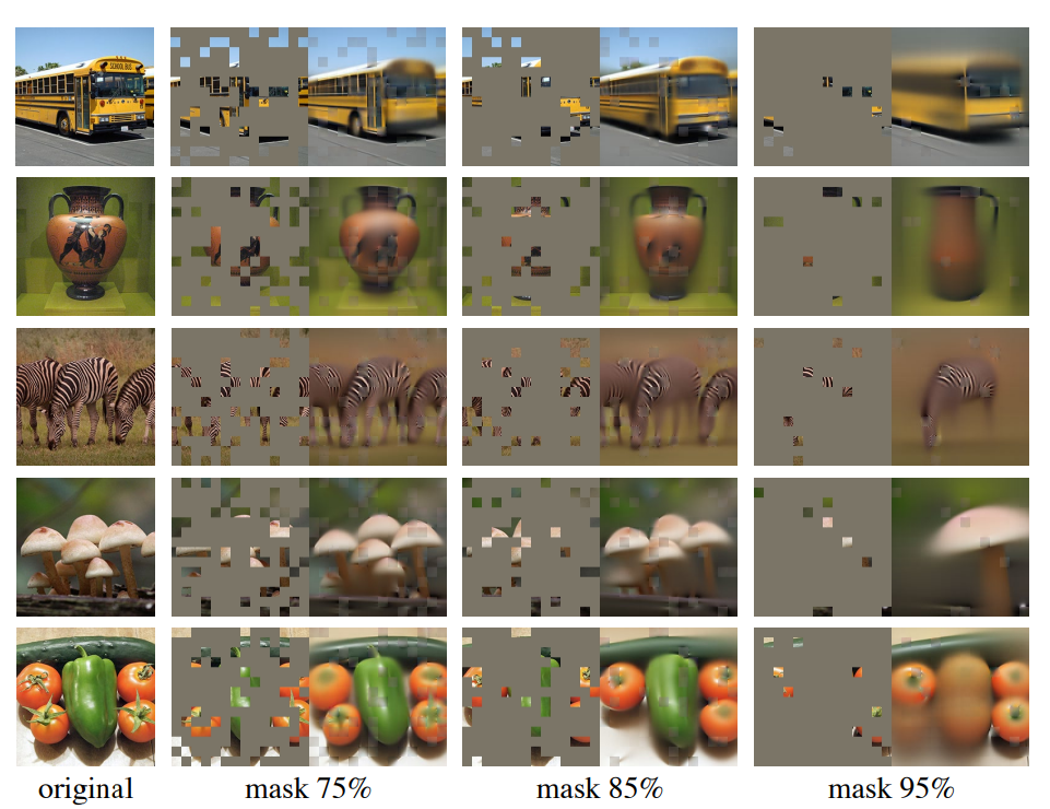
In the image processing field, a good example comes from “Masked Autoencoders Are Scalable Vision Learners” [7]. It shows how an efficient masking strategy using grayed out image patches can bring both greater generalization capabilites and better scalability.
Figure on the right comes from the paper and shows image reconstruction capabilities using different masking ratios.
These techniques can also be used in control-related problems. The intuition would be to hide part of a trajectory (actions, observations), so that the model learns to reconstruct it. Again, the model would learn system dynamics by guessing what action(s) and/or observation(s) led to a specific state. Obsiously, the difficulty increases with the size of the mask.
The main difference with “Inverse dynamics prediction” here will stand in the mask itself: instead of predicting a single action while hiding the future, we’ll let the model see it and predict the whole trajectory (or part of it). While the 2 technics seem pretty similar, their addition demonstrates benefits in model performance.
Here is an illustration of such trajectory with hidden actions but no future masking:

Let’s take a simple example where we want to mask the first 2 action tokens in a trajectory. Here is how the tokens should look like after masking them, given that -1 is used as a masking value.
o1 a1 o2  a2 o3 a3...
 1 -1  1  -1  1  1
 1 -1  1  -1  1  1
 1 -1  1  -1  1  1
 1 -1  1  -1  1  1
The implementation is quite straightfoward.
import torch
import numpy as np

# our dimensions
B, T, C = 4, 8, 1
# tokens that will be partially masked
masked_tokens = torch.ones((B, T, C))
# the index of vectors, here actions, that will be masked
mask_idx = [0, 1]
# masked token value
emb_mask_value = -1

for j in range(len(mask_idx)):
  # actions are at odd indices
  masked_tokens[:, 1 + 2 * mask_idx[j], :] = emb_mask_value
Result (reduced to 2 dimensions for the sake of clarity):
tensor([[ 1., -1.,  1., -1.,  1.,  1.,  1.,  1.],
        [ 1., -1.,  1., -1.,  1.,  1.,  1.,  1.],
        [ 1., -1.,  1., -1.,  1.,  1.,  1.,  1.],
        [ 1., -1.,  1., -1.,  1.,  1.,  1.,  1.]])
Closing the loop: loss computation
What’s next? Once we have our masked tokens, we’ll want to predict what we held out and compute our loss against actual targets.
Example below builds on previous “random trajectory masking” output and compute such loss.
from torch.nn import functional as F

# this is a pass-all-through mask (only ones), so attention blocks can see in the future
noop_mask = torch.ones((B, T, C))
# forward pass on multi-head attention blocks (not define here for brevity)
# masked_tokens is defined in previous example
x = attn_blocks((masked_tokens, noop_mask))
# forward pass on a prediction head, typically a set of linear layers
logits = pred_head(x[:, mask_idx, :])
# actual targets
action_targets = actions[:, mask_idx, :]
# loss computation. MSE used for continuous actions, cross entropy for discrete ones
loss = F.mse_loss(logits, action_targets)
If we have multiple pre-training objectives, we can simply add up the losses together and optimize a single loss, for a complex and informative control-oriented pre-training task.
For instance, let’s say we have an inverse dynamics prediction and random masking as pre-training objectives. There respective losses would be $L_{inv}$ and $L_{rnd}$. The total loss that we’d aim to minimize would then be $L_{tot} = L_{inv} + L_{rnd}$
Conclusion and opportunities
In this article we’ve seen how masking can be used for representation learning in self-supervised pre-training. Through simple masking examples, we’ve seen how a model can learn how a system behaves. Masking is a versatile technique, and designing expressive and system-specific objectives should be possible using this technique.
These concepts, inherited from the NLP and vision fields, are certainly key to create decision foundation models, which learn important dynamics of the systems at hand and can produce accurate trajectories for modeling downstream tasks like control policies. With robust foundation models, it would then be possible to train policies using a variety techniques, including but not limited to RL. Imitation learning (IL) or Model Predictive Control (MPC) can as well take advantage of the generative nature of the pre-trained model.
References
[1] Huang, Shengyi and Ontañón, Santiago. A Closer Look at Invalid Action Masking in Policy Gradient Algorithms. 2022
[2] Adil Zouitine. Masking in Deep Reinforcement Learning. 2022
[3] Emilio Parisotto and H. Francis Song and Jack W. Rae and Razvan Pascanu and Caglar Gulcehre and Siddhant M. Jayakumar and Max Jaderberg and Raphael Lopez Kaufman and Aidan Clark and Seb Noury and Matthew M. Botvinick and Nicolas Heess and Raia Hadsell. Stabilizing Transformers for Reinforcement Learning. 2019
[4] Tianwei Ni and Michel Ma and Benjamin Eysenbach and Pierre-Luc Bacon. When Do Transformers Shine in RL? Decoupling Memory from Credit Assignment. 2023
[5] Lili Chen and Kevin Lu and Aravind Rajeswaran and Kimin Lee and Aditya Grover and Michael Laskin and Pieter Abbeel and Aravind Srinivas and Igor Mordatch. Decision Transformer: Reinforcement Learning via Sequence Modeling. 2021
[6] Jacob Devlin and Ming-Wei Chang and Kenton Lee and Kristina Toutanova. BERT: Pre-training of Deep Bidirectional Transformers for Language Understanding. 2019
[7] Kaiming He and Xinlei Chen and Saining Xie and Yanghao Li and Piotr Dollár and Ross Girshick Masked Autoencoders Are Scalable Vision Learners. 2021
[8] Keiran Paster and Sheila McIlraith and Jimmy Ba You Can’t Count on Luck: Why Decision Transformers and RvS Fail in Stochastic Environments. 2022
[9] Adam Stooke and Kimin Lee and Pieter Abbeel and Michael Laskin. Decoupling Representation Learning from Reinforcement Learning. 2021
[10] Alex Lamb and Riashat Islam and Yonathan Efroni and Aniket Didolkar and Dipendra Misra and Dylan Foster and Lekan Molu and Rajan Chari and Akshay Krishnamurthy and John Langford. Guaranteed Discovery of Control-Endogenous Latent States with Multi-Step Inverse Models. 2022-arxiv 2022-blog
[11] Kate Rakelly and Abhishek Gupta and Carlos Florensa and Sergey Levine. Which Mutual-Information Representation Learning Objectives are Sufficient for Control?. 2021
[12] Yanchao Sun and Shuang Ma and Ratnesh Madaan and Rogerio Bonatti and Furong Huang and Ashish Kapoor. SMART: Self-supervised Multi-task pretrAining with contRol Transformers. 2023
[13] Ashish Vaswani and Noam Shazeer and Niki Parmar and Jakob Uszkoreit and Llion Jones and Aidan N. Gomez and Lukasz Kaiser and Illia Polosukhin. Attention Is All You Need. 2017
[14] Andrej Karpathy. Let’s build GPT: from scratch, in code, spelled out. 2023